7.8 Plotter interaction
At times, it is convenient to use the state of the plotter as feedback to plotted expressions. This kind of feedback has been seen before, in §7.6, where axis domains were introduced. These are described further here, along with axis variables and a clipping function.
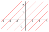
As seen in Figure §7.10 an axis domain generates a sequence of values running from
one end of an axis to the other in small steps that can be used to plot line segments. Axis domains
are accessed using the simple notation 

The ends of the axes can be changed in the plotter. For some plotted functions, it may be desirable to somehow bind the
function to the axes so the plot can reflect changes in the axes. This is accommodated by
making the ends of the axes available via the axis-end variables 


Another facility that interacts with the state of the plotter is a special line function that
draws a line clipped to the region defined by the axes. This is not always necessary because many
plots are composed of small line segments that are clipped by simply comparing their two end-points to
the plot region. But for a general line where only the segment that crosses the plot region is
to be viewed, the line-clipping function is used to constrain the displayed segment.
That is, only points that fall within the region bounded by the lines 


The line-clipping function is parameterized by two row vectors. The first defines a point on the line. The
second provides the line's attitude. Together, the point and the attitude provide a
parametric specification of a line. For example, the line 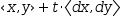
The line function is parameterized by a point and an attitude.
As a non-trivial example, consider the problem of drawing lines from the family